§ TL;DR
Token generation timing leaks model architecture and optimizations
Model architecture is a trade secret. So is the way a provider serves it: which optimizations run in the inference pipeline, and how they are configured.
However, the stream of generated tokens naturally includes the arrival time of every [group of] token(s). We show that those arrival times, measured through an ordinary chat interface or API, recover both kinds of secret.
The first attack recovers deployment details: which inference optimizations a provider is running, and how they are configured. We use speculative decoding as a proof of concept to demonstrate it. On Google's Gemini Flash 2.5 the attack recovers a hidden draft model with a 128K context window. Flash 2.5 Lite matches it, and Flash 1.5 comes in at 32K. None of this is documented anywhere.
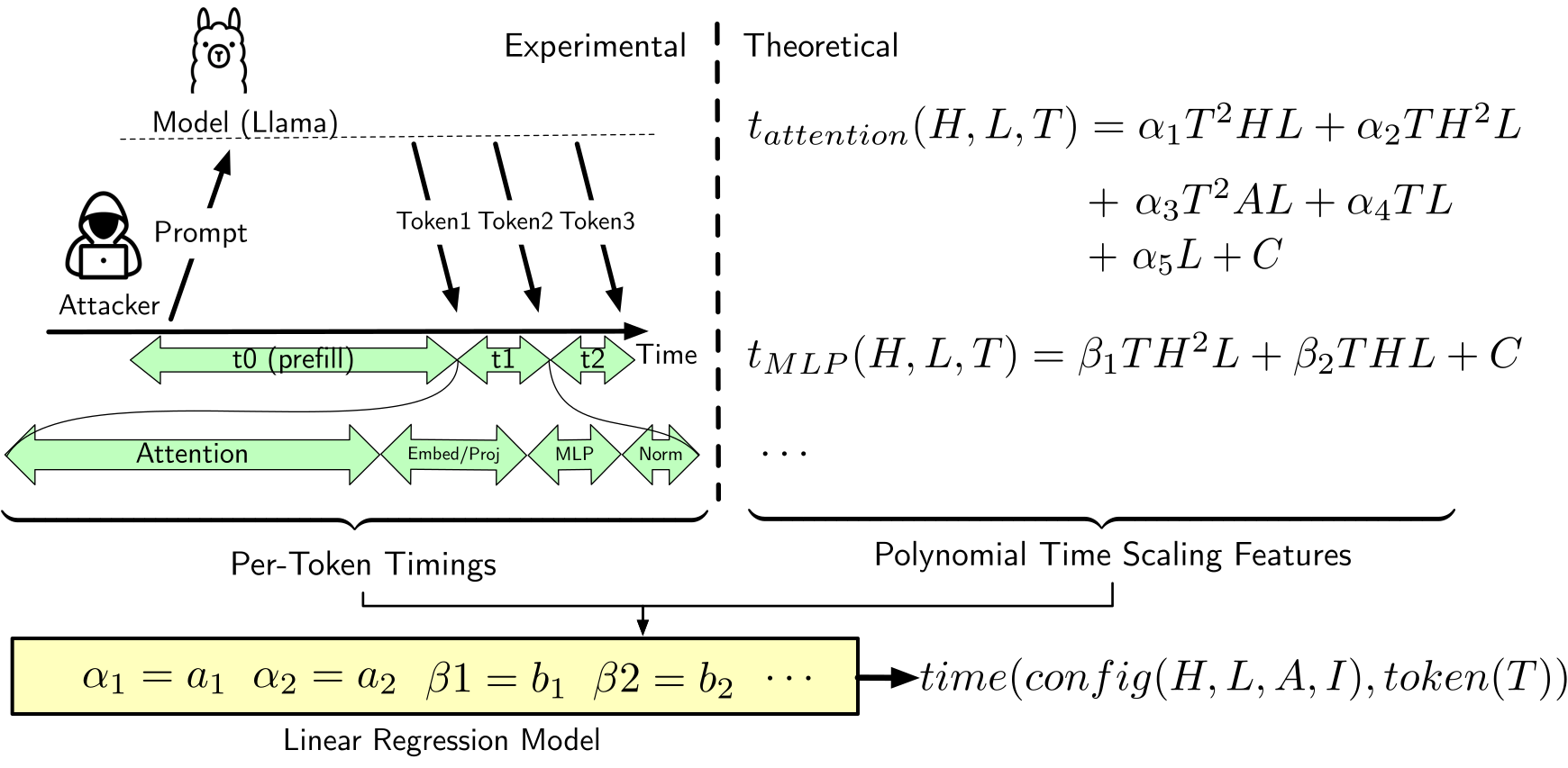
The second attack recovers the architecture itself: how deep the model is, how wide, and how many attention heads it has. The reasoning is that those choices impact how much arithmetic each generated token costs, and arithmetic costs time. We derive that relationship for a transformer running on a GPU, calibrate its constants against measurements we collect ourselves, and end up with a predictor that turns any candidate architecture into the timing curve it would produce. Recovering an unknown model then becomes a search: enumerate the plausible configurations, predict a curve for each, and keep the ones that match what was measured. We ran this against a Llama 3.1 8B model hosted on Weights & Biases' inference service and treated as a black box, and the correct hidden dimension came back ranked first.
§ Background
What's actually being streamed
A hosted model does not give you a complete response all at once. It gives you one or a few tokens, then more, and the interval between them is proportional to how long the GPU took to produce them. Providers work to keep those intervals short, because users don't want to wait. A pipeline tuned that carefully ends up publishing a high-resolution trace of its own behavior to anyone willing to timestamp the arrivals.
What sets the size of an interval? Some of it is the network. The rest is the model and the machine under it: how many matrix multiplications one forward pass needs, how big each one is, how much memory traffic they generate, and which optimizations the provider is running underneath.
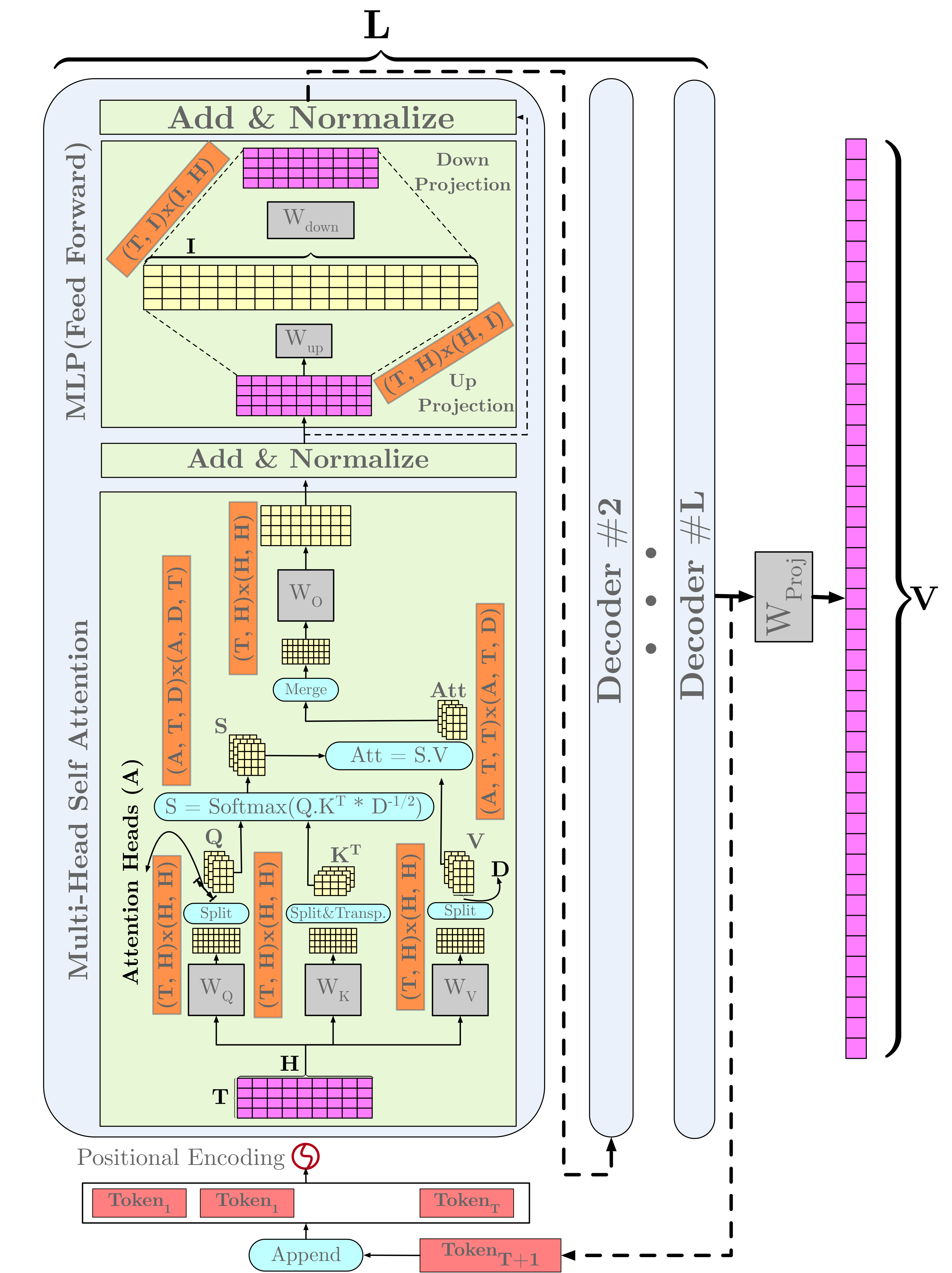
Those quantities are not arbitrary. For a decoder-only transformer, nearly all of the per-token cost is set by five numbers:
- H is the hidden dimension, the width of the vector carried through the network.
- L is the number of decoder layers, the depth.
- A is the number of attention heads.
- I is the intermediate size of the MLP.
- T is the sequence length.
The first four are the architecture, and providers treat them as confidential. The fifth is the prompt, and it belongs to the attacker. That asymmetry is what the attack exploits: sweep T across a wide range, watch how per-token latency responds, and work backwards to the four numbers you cannot see.
Network latency is the obvious objection, and it is smaller than it looks. A constant round-trip time shifts every arrival by the same amount, which leaves the differences between consecutive tokens untouched. Only the variance matters. Over the endpoints we measured it is small: mean RTT of 26.65 ms to Gemini with a standard deviation of 0.07 ms. Standard deviation sits under 5% of the fastest per-token generation time we recorded. The signal survives the network.
§ Threat model
The attacker in this work is a customer
They open an account, send prompts through the documented streaming endpoint, and record when each token arrives. That is the whole apparatus. No logits, no activations, no server logs, no privileged position on the network, no access to the machine. They know what the provider's documentation tells everyone: the model's name, its family, its advertised context length. Nothing more about what runs underneath.
The attacker has
- A standard API account with streaming enabled
- A timer
- Public documentation: model name, family, advertised context length
- Control over the content and length of their own prompts
The attacker does not have
- Logits, logprobs, or activations
- Server logs or system-level access
- Any privileged network position
- Control over generation parameters beyond what the API exposes
What they're after: the number of decoder layers (L), hidden dimension (H), attention heads (A), and MLP intermediate size (I), plus which inference optimizations are running and how they are configured.
Both attacks work from exactly this position. They differ in what they extract, not in what they are allowed to see: the same stream, the same timer.
Recovering the architecture needs one thing more. Predicting how long a candidate configuration would take requires a model of the hardware it would run on, so there we also assume the attacker knows the GPU class serving the target and can obtain the same class to calibrate against, and that the model is served from a single GPU for now. We leave Multi-GPU serving, which is how the largest frontier models actually run, to future work.
That one assumption is why the architecture results come from small and mid-size models on known hardware. The Gemini results that follow need nothing beyond the interface and a timer.
§ Attack 1
Detecting inference optimizations
Serving a model at scale is not just a matter of running it. Providers serve it through a pipeline of optimizations chosen to cut latency and cost: caching, batching, quantization, scheduling, speculation. Any optimization that makes some tokens cheaper changes how long those tokens take, and anyone timing the stream can see this dependency. In principle an attacker can probe for any of them. We demonstrate the idea with an attack on speculative decoding.1
The optimization is simple and it works. Run a small draft model ahead of the large one. The draft proposes several tokens. The large model verifies them all in a single forward pass. If the draft guessed right, several tokens are accepted at once and the expensive model ran once instead of four times. If it guessed wrong, the speculated tokens are discarded and the pipeline falls back to producing a single token the slow way, plus the wasted draft work.
Processor designers have been here before. This is speculative execution, and part of why Spectre2 worked is that speculation which gets rolled back still leaves a trace. Speculative decoding does not make every token faster. It makes the common case faster and the uncommon case slower. That difference is visible from outside the API.
Making the draft model fail on purpose
Detecting some optimization is easy. Any input-dependent variation in per-token latency tells you something is running. Attributing that variation to speculative decoding specifically is the hard part.
The lever is the draft model's context window. A draft model is picked to be small and fast, and extending its context costs both compute and memory, so in practice it gets a shorter window than the model it serves. That gives us a prompt length at which the draft goes blind and the main model does not. Past it, the draft is guessing at information it cannot read, so every speculation is rejected, not occasionally but every time.
The prompt puts a random number at the very front and pushes it back with padding:
The value of number NUM at the start was equal to
The task never gets harder. It is the same recall task at every length, so prompt length is the only thing that varies. Two details matter beyond that. The number and the padding are freshly randomized on every trial, which stops server-side caching from answering for us. And prompt lengths are sent in randomized order, so a provider that throttles by length or request sequence cannot be mistaken for a cliff.
Checking the instrument first
Before pointing this at a production API, we pointed it at a system where we already knew the answer. Llama 2 13B as the main model, TinyLlama 1.1B as the draft, running a public implementation of speculative decoding on a local GPU.
Sweeping prompt length from 82 to about 4,000 tokens, per-token latency is flat and low, and then it jumps. Binary search puts the jump at Tbreak = 2,030 tokens. Subtracting the prologue leaves 2,018. Round to the nearest power of two, since context windows essentially always are one, and the estimate is 2,048.
TinyLlama 1.1B has a 2,048-token context window. Turning speculative decoding off removes the jump entirely, which rules out the obvious alternative explanation.

The same procedure against Gemini
Unmodified, against Google's public API. Gemini Flash 2.5 shows the cliff at a prompt length of 131,059 tokens. Below it, tokens arrive in 1.7 to 3.6 milliseconds. Above it, 8.0 to 11.2. Averaged across the four output positions we tracked, crossing the break multiplies per-token latency by 3.2×. Subtract the 17-token prologue and the draft model's context window is 131,042 tokens, or 128K less a 30-token margin.
Flash 2.5 Lite breaks at the same place. Flash 1.5 breaks at 32,743, which is 32K. Google documents none of this.


| System | Measured break | Recovered draft context |
|---|---|---|
| Llama 2 13B + TinyLlama 1.1B (local) | 2,018 | 2K ✓ |
| Gemini Flash 2.5 | 131,042 | 128K |
| Gemini Flash 2.5 Lite | 131,042 | 128K |
| Gemini Flash 1.5 | 32,743 | 32K |
- Prompt
- 130,939 tokens
- Measured
- Regime
131,059 − 17 (prologue) = 131,042 ≈ 128K , the draft model's context window.
What the test cannot see
The test detects a draft model whose context window is shorter than the main model's. A provider running a draft model with a matched window would be invisible to it, as would a deployment that speculates in some other way. This method produces false negatives by construction. Where we saw no step, "we did not detect it" is the strongest claim available.
§ Attack 2
Reading architecture off the timings
In a basic transformer, per-token generation time grows with sequence length, roughly quadratically, because attention is quadratic in T.
Write that growth as a quadratic in T and it has three coefficients: one multiplying T², one multiplying T, and a constant. Those coefficients are not free parameters. Each one traces back to a particular matrix multiplication inside the model, and the size of that multiplication is fixed by the architecture. Adding layers scales some terms and leaves others alone. Widening the hidden dimension scales a different set again. So the four numbers we are after, H, L, A and I, determine the three coefficients, and the coefficients determine the shape of the curve. Two models with different architectures produce differently-shaped curves, and the shape is a fingerprint.

A timing model you can read
We build the predictor bottom-up. Decompose a decoder block into its subcomponents, then each subcomponent into primitive operations: matrix multiplications, softmax, elementwise adds. Derive each primitive's compute and memory cost analytically as a function of T, H, A, I and the element width. Convert cost to time by dividing by the machine's peak arithmetic throughput and memory bandwidth. Then attach a coefficient to every term to absorb what the analysis does not capture: tiling, vectorization, kernel launch overhead, imperfect overlap between compute and memory.
For a single query projection that gives:
α, β and C come from regression on real measurements. Fit one model per subcomponent, sum them, and add a final regression for the residual overhead that belongs to no component in particular: kernel launches, synchronization, per-iteration costs.
Why linear regression, when a neural network would fit the data better? Because the terms correspond to real cost components, so a bad fit is diagnosable. Because linear models do not chase residual noise, which a more flexible model would absorb and then fail to extrapolate from. And because individual terms can be swapped when the implementation changes, which is exactly what happens next.
Four predictors
- EagerBaseline. Attention decomposed into cuBLAS matrix multiplications, as in a stock HuggingFace transformers forward pass.
- Eager (Corrected)Same, plus the cuBLAS kernel corrector below. This is the variant that survives contact with architectures it has not seen.
- Flash2Attention terms replaced with FlashAttention2's3 memory-access behavior. Derived from the algorithm, not from one implementation. Every other subcomponent is unchanged and simply refit.
- KV-Flash2Flash2 split into a prefill formulation and a decode formulation, because KV caching makes those two phases scale differently.
Modeling the library
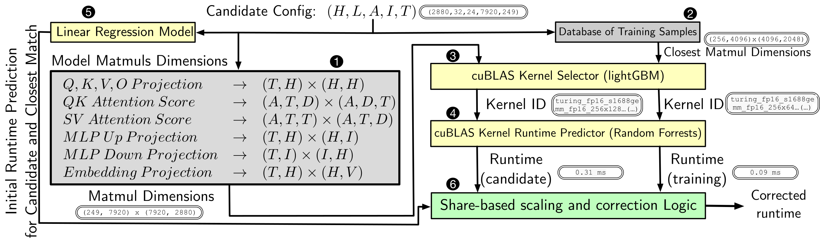
cuBLAS does not have one matrix-multiply kernel. It has many, and it chooses between them based on operand shapes and internal heuristics. A predictor whose coefficients were fit at one set of dimensions mispredicts at another, not because the asymptotics changed but because the library quietly switched to a different kernel with different constants.
So we model the library too. A LightGBM4 classifier predicts which kernel cuBLAS will select for a given pair of operand shapes, and a small random forest per kernel predicts that kernel's runtime.
On test architectures the predictor had never seen, this takes NRMSE from 0.411 to 0.119. The naive variant fits its training family fine and falls apart off it. The corrected variant holds.
Under the hood: the search space
A grid over every integer configuration would be hopeless, so the space is pruned with conventions real models follow. Layer counts are integers in a plausible band. Hidden dimensions are multiples of a base stride, 64 or 128. Head count is constrained so per-head dimension divides the hidden size evenly. Combinations that no one builds, like a very deep model with a tiny hidden size, are dropped.
That leaves 1,540 candidate configurations for the main evaluation, scored against each of 130 target configurations. The whole search takes about 20 minutes across 40 CPU cores. Candidates are ranked by RMSE between their synthesized trace and the observed one, and we keep a shortlist rather than the single best match, because timing is noisy and nearby configurations can look alike under a limited set of prompts.
A retrieval counts as correct only if every targeted parameter lands within one step of the truth: one layer for L, 128 for H, 4 for A, 1024 for I.
Results
Recovering one parameter with the others fixed works well across all three implementations. Recovering both at once is markedly harder, and the reason is visible in the model: most terms depend on the product H·L, so the classifier has to separate effects the physics has already mixed.
| Target | Eager (Corrected) | Flash2 | KV-Flash2 |
|---|---|---|---|
| Layers (L) | 86.15 | 97.69 | 83.78 |
| Hidden dim (H) | 71.54 | 100.00 | 70.95 |
| Both (H, L) | 65.38 | 54.62 | 45.27 |
The predictor also transfers across model families it was never trained on. Trained on Llama 3.2 1B alone, it predicts Qwen2.5 1.5B, Phi-3.5-mini 3.8B and Gemma2 2B with NRMSE between 0.159 and 0.186, comparable to its error on the family it learned from.
| Test model | NRMSE | L | H | (H, L) |
|---|---|---|---|---|
| Llama 3.2 1B | 0.221 | 100.00 | 93.64 | 90.91 |
| Llama 3.2 3B | 0.119 | 86.15 | 71.54 | 65.38 |
| Qwen2.5 1.5B | 0.159 | 77.27 | 100.00 | 50.00 |
| Phi-3.5-mini 3.8B | 0.183 | 97.50 | 97.50 | 80.00 |
| Gemma2 2B | 0.186 | 100.00 | 77.50 | 47.50 |
Against a real endpoint
Everything above runs on hardware we control. The last experiment does not. We pointed the attack at Weights & Biases' Llama 3.1 8B Instruct streaming API. That is a machine we have no access to, an inference stack we did not choose and did not instrument, timed by the same client we used for the Gemini experiments.
With L fixed, the correct hidden dimension ranks first. With H fixed, the correct layer count ranks fourth. Searching both at once across 2,068 configurations, a near-match at (H=4096, L=34) ranks 8th and the true configuration (H=4096, L=32) ranks 28th.

Limitations
The W&B result deserves an honest reading. It is a model from a family the predictor was trained on, though at dimensions outside its training range, served in FP16 on hardware whose class we knew. It shows the pipeline survives contact with a real API. It does not show that a frontier model is currently recoverable at this stage.
Three limits are worth stating plainly. Recovering H and L jointly drops to 45–65% even in the top five. The Flash2 and KV-Flash2 predictors are less accurate than the eager one. FlashAttention2's kernel is fused and its behavior depends on more than the dominant memory term we model, and that error propagates straight into ranking accuracy. And once a KV cache is warm, the decoding phase carries very little architectural signal, which is why the remote attack leans mostly on prefill.
§ Mitigations
Every mitigation trades against the latency it was meant to save
Make per-token time constant. Pad every token's generation to the worst case so latency stops depending on the architecture or on what the pipeline did. This closes the channel completely. It also means running every request at worst-case speed, which can be several times slower and deletes the reason the optimizations were deployed.
Buffer the stream. Emit tokens in fixed-size groups at fixed intervals rather than the moment each one is ready. This coarsens the channel instead of removing it, and it is adjustable, since larger groups leak less. The cost lands on time-to-first-token and on how responsive the stream feels, which is exactly the metric providers tune streaming for.
We do not have a mitigation that is free. The channel exists because inference is optimized and results are streamed as they arrive. Both are deliberate product decisions, and the defenses trade directly against them.
§ Responsible disclosure
Disclosure
- 2025-11-07Speculative decoding attack and the Gemini findings disclosed to Google.
- 2026-01-29Google acknowledged the findings.
This page describes what we found and why it matters. It is not a how-to, and it adds no operational detail beyond what the paper reports.
§ References
References
Works cited above, as they appear in the paper's bibliography. The full reference list is in the paper.
- Y. Leviathan, M. Kalman, and Y. Matias. Fast inference from transformers via speculative decoding. Proceedings of the 40th International Conference on Machine Learning (ICML'23), 2023.
- P. Kocher, J. Horn, A. Fogh, D. Genkin, D. Gruss, W. Haas, M. Hamburg, M. Lipp, S. Mangard, T. Prescher, M. Schwarz, and Y. Yarom. Spectre attacks: exploiting speculative execution. 40th IEEE Symposium on Security and Privacy (S&P'19), 2019.
- T. Dao. FlashAttention-2: faster attention with better parallelism and work partitioning. arXiv:2307.08691, 2023.
- G. Ke, Q. Meng, T. Finley, T. Wang, W. Chen, W. Ma, Q. Ye, and T.-Y. Liu. LightGBM: a highly efficient gradient boosting decision tree. Proceedings of the 31st International Conference on Neural Information Processing Systems (NIPS'17), pages 3149–3157, 2017.
§ Citation
Cite this work
@article{majidi2026leakylms,
  title   = {Leaky Language Models: Stealing Architecture and Inference
             Optimizations via Per-Token Timing},
  author  = {Majidi, Sadegh and Mireshghallah, Niloofar and Taram, Kazem},
  journal = {arXiv preprint arXiv:2607.20723},
  year    = {2026}
}
Code, measurement scripts and analysis notebooks are in the artifact repository, organized to mirror the structure of the paper.
§ Acknowledgments
Acknowledgments
This blog post was generated from our article, with a lot of help from Claude.
Supported by Longview Philanthropy. Correspondence to mmajidiy@purdue.edu.